The tutorial shows how to create a repayment plan in Excel to detail regular payments for a repayment loan or mortgage.
An amortizing loan is just a fancy way to define a loan that is paid back in installments throughout the life of the loan.
Basically all loans amortize in one way or another. For example, a fully amortizing loan for 24 months has 24 equal monthly payments., Each payment relates a certain amount to the principal and a part to the interest. To detail each payment for a loan, you can create a loan amortization schedule.
An amortization schedule is a table that lists periodic payments on a loan or mortgage over time, breaks down each payment into principal and interest, and shows the remaining balance after each payment is made.,
- How to create an amortization schedule for loans in Excel
- Repayment schedule for a variable number of periods
- Repayment schedule for loans with additional payments
- Excel – Repayment template
How to create an amortization schedule for loans in Excel
To create a loan or mortgage amortization schedule in Excel, we need to use the following functions:
- PMT function-calculates the total amount of a regular payment. This amount remains constant throughout the life of the loan.,
- PPMT function-Retrieves the principal portion of each payment that goes toward the loan principal, i.e., the amount you borrowed. This amount increases for subsequent payments.
- IPMT function-finds the interest part of each payment that goes towards interest. This amount decreases with each payment.
Now let's go through the process step by step.,
Set up the amortization table
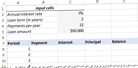
First define the input cells where you enter the known components of a loan:
- C2 – annual interest rate
- C3 – Loan term in years
- C4 – number of payments per year
- C5 – Loan amount
Next, create an amortization table with the labels (period, payment, interest, principal)., Balance) in A7:E7., In the Period column, enter a series of numbers equal to the total number of payments (1 – 24 in this example):
With all the components known, we come to the most interesting part – credit amortization formulas.
Calculate total payment amount (PMT formula)
The payment amount is calculated using the function PMT(rate, nper, pv, , ).
To correctly handle different payment frequencies (z. B. weekly, monthly, quarterly, etc.).,), it should be consistent with the given values for rate and nper arguments:
- Rate – divide the annual interest rate by the number of payment periods per year ($C$2/$C$4).
- Nper-multiply the number of years by the number of payment terms per year ($C$3*$C$4).
- For the argument pv, enter the loan amount ($C$5).
- The arguments fv and type can be omitted, since their default values work fine for us (balance after last payment should be 0; payments are made at the end of each period).,
Putting the above arguments together, we get this formula:
Please note that we use absolute cell references, as this formula should be copied into the following cells without any modifications.,
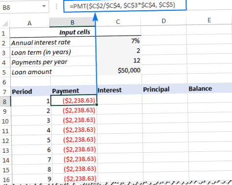
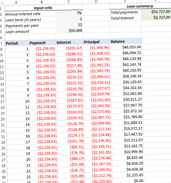
Enter the PMT formula in B8, drag it down the column, and you will see a constant payment amount for all the periods:
Calculate interest (IPMT formula)
To find the interest portion of each periodic payment, use the IPMT(rate, pro, nper, pv, , ) function:
All arguments are the same as in the PMT formula, except for the argument per, which specifies the payment period., This argument is given as a relative cell reference (A8) because it should change based on the relative position of a row into which the formula is copied.,
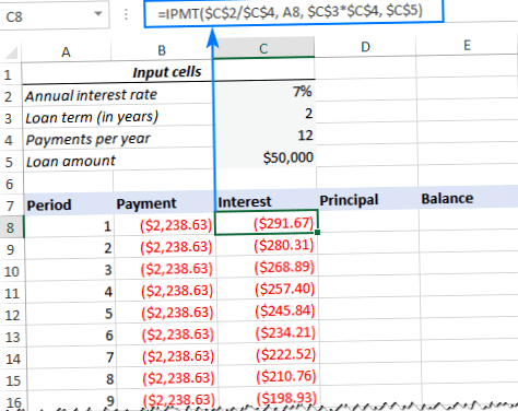
This formula goes to C8, and then copy it to as many cells as necessary:
Find principal (PPMT formula)
To calculate the principal balance of each periodic payment, use this PPMT formula:
The syntax and arguments are exactly the same as discussed in the IPMT formula above:
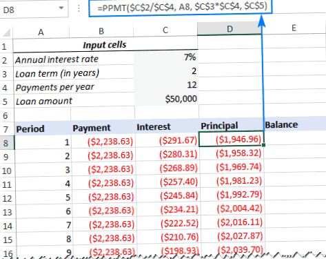
This formula goes to column D, starting in D8:
Tip. To verify that your calculations are correct at this time, add up the numbers in the Principal and Interest columns., The total should equal the value in the payment column in the same row.
Get the remaining amount
To calculate the remaining amount for each period, we use two different formulas.
To find the balance after the first payment in E8, add the loan amount (C5) and the principal of the first period (D8):
Since the loan amount is a positive number and the principal is a negative number, the latter is actually subtracted from the former.,
For the second and all subsequent periods, add the previous balance and the principal value for that period:
The above formula is E9 and copy it to the column. Because of the use of relative cell references, the formula adjusts correctly for each line.
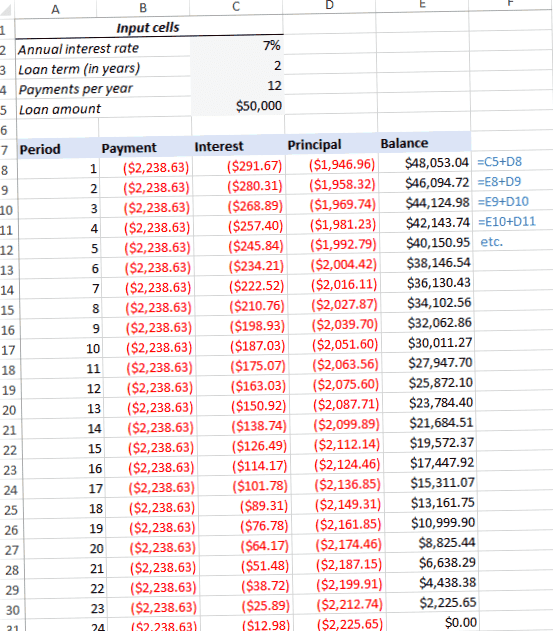
This was ' s! Our monthly loan repayment schedule is ready:
Tip: return payments as positive numbers
As a loan is disbursed from your bank account, Excel functions return the payment, interest, and principal as negative numbers., By default, these values are highlighted in red and enclosed in parentheses, as you can see in the image above.
If you prefer to have all results as positive numbers, put a minus sign in front of the PMT, IPMT and PPMT functions.
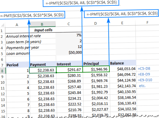
Use subtraction instead of addition for the balance formulas, as shown in the screenshot below:
Amortization schedule for a variable number of periods
In the above example, we have created an amortization schedule for the predefined number of payment periods., This quick one-time solution works well for a specific loan or mortgage.
If you want to create a reusable amortization schedule with a variable number of periods, you need to take a more comprehensive approach, which is described below.
Enter the maximum number of periods
In the column Period, insert the maximum number of payments you would like to allow for a loan, z. B. from 1 to 360. You can use Excel's AutoFill feature to enter a range of numbers more quickly.,
Use IF statements in amortization formulas
Now that you have many excessive period numbers, you need to somehow limit the calculations to the actual number of payments for a given loan. This can be done by wrapping each formula in an IF statement. The logical test of the IF statement checks if the period number in the current row is less than or equal to the total number of payments. If the logical test is TRUE, the corresponding function will be calculated; if FALSE, an empty string will be returned.,
If period 1 is in row 8, enter the following formulas in the appropriate cells and then copy them into the entire table.,
For period 1 (E8), the formula is the same as in the previous example:
For period 2 (E9) and all subsequent periods, the formula takes this form:
As a result, you have a correctly calculated amortization schedule and a number of empty rows with the period numbers after the loan is disbursed.,
Hide extra periods numbers
If you can live with a series of redundant period numbers displayed after the last payment, you can look at the work done and skip this step. If you're striving for perfection, hide any unused periods by setting a conditional formatting rule that sets the font color to white for all rows after the final payment.,
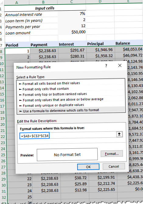
Select all data rows from your amortization table (in our case A8:E367) and click Start tab> Conditional Formatting> New Rule…> Use a formula to determine which cells to format.
In the appropriate field, enter the following formula that checks if the period number in column A is greater than the total number of payments:
Important note!, For the conditional formatting formula to work correctly, be sure to use absolute cell references for the loan term and payments per year cells you are multiplying ($C$3*$C$4). The product is compared to the period 1 cell for which you use a mixed cell reference – absolute column and relative row ($A8).
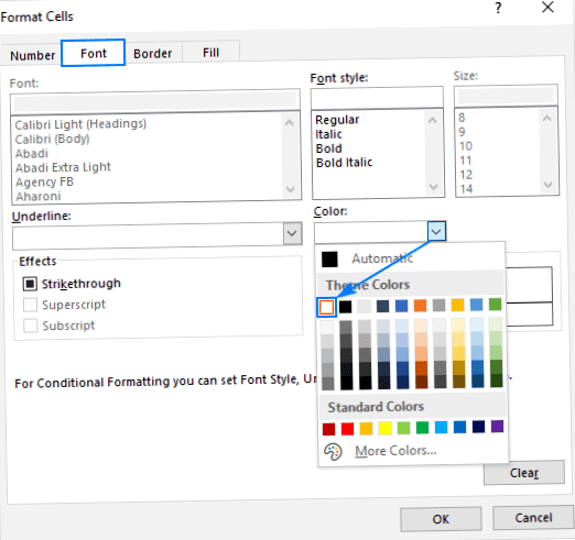
Then click the Format… button and select the white font color. Ready!,
Make a credit summary
To view summary information about your loan at a glance, add a few more formulas at the top of your repayment schedule.
Total Payments (F2):
Total Interest (F3):
If you have payments as positive numbers, remove the minus sign from the above formulas.
That was it! Our loan amortization schedule is complete and good to go!,
Download loan amortization schedule for Excel
How to create an amortization schedule for loans with additional payments in Excel
The amortization schedules described in the previous examples are easy to create and follow (hopefully :). However, you are leaving out a useful feature that many loan payers are interested in – additional payments to pay off a loan faster. In this example, we'll look at how to create an amortization schedule for loans with additional payments.
Define input cells
Begin as usual by setting up the entry cells., In this case, we call these cells as described below to make it easier to read our formulas:
- interestRate – C2 (annual interest rate)
- LoanTerm – C3 (loan term in years)
- PaymentsPerYear – C4 (number of payments per year)
- LoanAmount – C5 (total loan amount)
- ExtraPayment – C6 (additional payment per period)
Calculate a scheduled payment
Apart from the input cells, our further calculations require one more predefined cell – the planned payment amount, d.h., the amount to be paid on a loan if no additional payments are made. This amount is calculated using the following formula:
=IFERROR(-PMT(InterestRate/PaymentsPerYear, LoanTerm*PaymentsPerYear, LoanAmount)"")
Please make sure that we put a minus sign in front of the PMT function to get the result as a positive number. To avoid errors if some of the input cells are empty, we include the PMT formula in the IFERROR function.
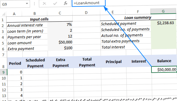
Enter this formula into a cell (in our case G2) and name this cell ScheduledPayment.,
Set up the repayment table
Create an amortization table for loans with the headings shown in the following screenshot. Enter a series of numbers beginning with zero in the Period column (you can hide the Period 0 row later if needed).
If you want to create a reusable repayment schedule, enter the maximum number of payment periods possible (0 to 360 in this example).
For period 0 (in our case, line 9), draw the balance value that corresponds to the original loan amount., All other cells in this row is left blank:
4. Create formulas for the amortization schedule with additional payments
This is an important part of our work. Since Excel's built-in functions don't provide for additional payments, we have to do all the math ourselves.
Hint:. In this example, period 0 is in row 9 and period 1 is in row 10. If your amortization table starts in a different row, adjust the cell references accordingly.,
Enter the following formulas on line 10 (period 1) and then copy them down for all remaining periods.
Scheduled Payment (B10):
If the scheduled payment amount (cell G2) is less than or equal to the remaining amount (G9), use the scheduled payment. Otherwise, add the balance and interest for the previous month.
As an extra precaution, we wrap this and all subsequent formulas in the IFERROR function., This prevents a number of different errors if some of the input cells are empty or contain invalid values.
Use an IF formula with the following logic:
If the extra payment amount (called cell C6) is less than the difference between the remaining balance and the principal of that period (G9-E10), return ExtraPayment; Otherwise, use the difference.
Tip. If you have variable additional payments, simply enter the individual amounts directly into the Additional Payment column.,
Just add the scheduled payment (B10) and the additional payment (C10) for the current period:
If the scheduled payment for a given period is greater than zero, return a smaller of the two values: scheduled payment less interest (B10-F10) or the remaining balance (G9); otherwise, return zero.
=IFERROR(IF(B10>0, MIN(B10-F10, G9), 0)"")
Please note that the principal includes only the part of the scheduled payment (not the additional payment!) this goes in the direction of the lender.,
If the scheduled payment for a given period is greater than zero, divide the annual interest rate (called cell C2) by the number of payments per year (called cell C4) and multiply the result by the balance remaining after the previous period; Otherwise, return 0.
=IFERROR(IF(B10>0, InterestRate/PaymentsPerYear*G9, 0)"")
If the balance (G9) is greater than zero, subtract the principal payment (E10) and the additional payment (C10) from the balance remaining after the previous period (G9); otherwise, return 0.,
=IFERROR(IF(G9>0, G9-E10-C10, 0)"")
Notice:. Because some of the formulas refer to each other (not a circular reference!), you may be showing incorrect results in the process. So don't start troubleshooting until you have entered the very last formula into your amortization table.
If everything is done correctly, your loan repayment schedule at this point should look something like this:
Hide extra periods
Set up a conditional formatting rule to hide the values in unused periods, as explained in this tip.,Payments per year:
Actual number of payments:
Count cells in the total payment column that are greater than zero, beginning with period 1:
Total Additional Payments:
Add cells in the additional payment column, starting with period 1:
Add cells in the interest column, starting with period 1:
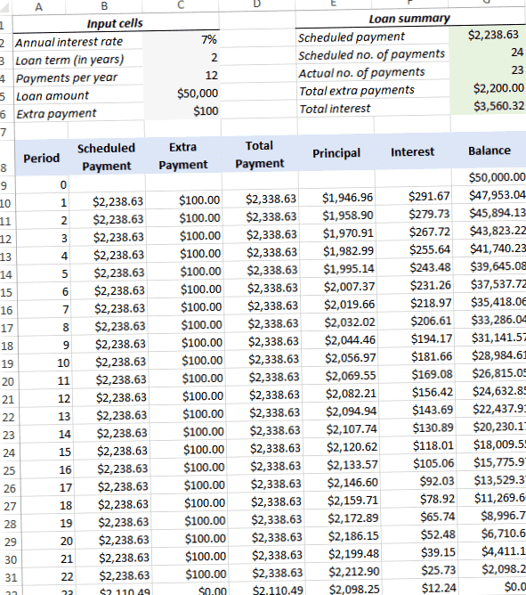
Optionally, you can hide the Period 0 row, and your amortization schedule for loans with additional payments is ready to go!, The screenshot below shows the final result:
Download loan amortization schedule with extra payments
Amortization schedule Excel template
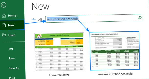
To create a top-notch loan amortization schedule in no time, use Excel's built-in templates. Just go to the file> New, type "amortization schedule" in the search box and select the template you want to use, e.g. B. these with additional payments: